Resource management

Economic exchanges

Land-use dynamics

Role-playing games

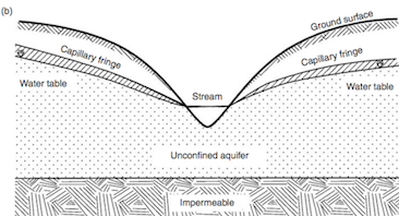
Demo_Aquifer: the ground water diffusion in an aquifer

Pierre Bommel, Bruno Bonté, Marie-Paule Bonnet, Grégoire Leclerc.

The aim of this model (zipfile, 191Ko) is to simulate water exchange between surface soil, river network and the underlying aquifer.
This model is a replication of the model by (Ravazzani et al. 2011) called MACCA-GW (for MACroscopic Cellular Automata for GroundWater).
It represents the water flow in unconfined aquifers. The model is based on a uniform regular lattice, that discretizes the water flow in space and time.
Many complex macroscopic fluid dynamical phenomena seem difficult to be modelled by cellular automata, because they take place on a large space scale and require a macroscopic level of description.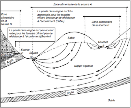

fig ANdrimont 1910

Groundwater flow systems; picture presented at the Brussels World Exhibition in 1910 by René d’Andrimont (from Jacobus J. de Vries in Delleur 1998).

The Demo_Aquifer model focuses only on unconfined aquifer: case b of the following figure:

Kinds of aquifers. (a) Confined aquifer; (b) unconfined aquifer. (from Delleur 1998). The Demo_aquifer model refers only on the unconfined aquifer (b).

The physical model based on the Darcy's law (1856)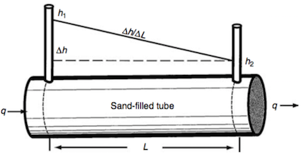

Figure illustrating tube experiments of Henri Darcy (from Delleur 1998).

The Darcy equation is:

Q=KA{\frac {\Delta H}{L}}

(eq. 1)

where :

Q : the volumetric flow rate (m³/s).
K : the hydraulic "conductivity" or "permeability coefficient" of the porous medium (m/s), which depends on both the properties of the porous medium and the viscosity of the fluid.
A : the area of the section (m²)
ΔH is the difference between upstream and downstream piezometric heights (i = ΔH/L is the hydraulic gradient)
L is the length of the sample.

The Demo_Aquifer model differentiates the flows (sources + or sinks -) into two parts: (1) lateral water diffusion and (2) vertical water fluxes:

(a) Von Neumann

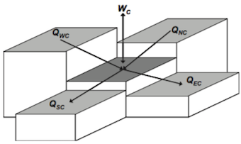(b)

(a) Scheme for the calculation of water fluxes between a central cell and its four adjacent cells. Qnc is the latteral flux coming from the northern cell, for example. Wc is the vertical flux representing source or sink (from Ravazzani et al. 2011). (b) flow between 2 cells.

Then the total incoming or outgoing flow is:
Q_C = Q_NC + Q_EC + Q_SC + Q_WC + W_C in [L³ T^-1], where

Q_NC + Q_EC + Q_SC + Q_WC represent the lateral water diffusion, and
W_C , the vertical water flows with the ground due to pumping wells (-) or recharge (+) by rain, river or lake.

According to Darcy equation (eq. 1), the water flux between central cell and, for example, northern cell, Q_NC is calculated as:
Qnc=(2TnTc)/(Tn+Tc) . (Hn-Hc)

(eq. 2)
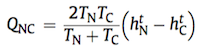
where:

T_N and T_C represent, respectively, the transmissivity [L² T^-1] of northern cell and central cell,
h^t_N and h^t_C represent, respectively, hydraulic head of northern cell and central cell at previous time step, t.

The flux Q_NC is positive if water is entering the central cell.
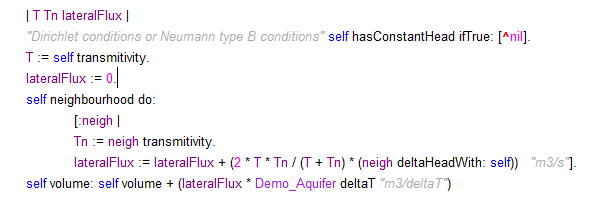
In Demo_Aquifer, the Transmitivity of a cell C is calculated as:
T_C = K_C . Z_C
where . Z_C is the thickness = (head - base) of the cell.

The term 2T_NT_C /(T_N + T_C) is the harmonic mean of transmissivity. It has been chosen because of its property to remove the impacts of large outliers by limiting the flux to the lower value of transmissivity.

The Reynolds number for determining the time step value

Darcy's law is only valid for slow, viscous flow as it is the case of most groundwater flows. Typically any flow with a Reynolds number less than 1 is clearly laminar, and it would be valid to apply Darcy's law. Experimental tests have shown that flow regimes with Reynolds numbers up to 10 may still be Darcian, as in the case of groundwater flow. The Reynolds number D (a dimensionless parameter) for porous media flow is defined as the ratio of physical and numerical diffusivities:
Reynolds nb

(eq. 3)
where :

ν is the hydraulic diffusivity of the aquifer. ν = = K.Z/S, in [L²/T] (= Transmissivity / storativity = conductivity . thickness / storativity)
(Δs)² is the area of the cell [L²]
Δt is the time step [T]

If we fix D = 1 to get stability, then the time step duration should be:
deltaT

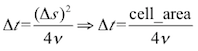(eq. 4)
So, in order to have smooth water movements, the model must first determine the duration of delta t, the minimum time step.

After calculating the diffusion flows between the cells, the hydraulic head of each cell is updated for the subsequent time step (t + Δt), applying the discrete mass balance equation: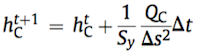

Ht+1=Ht + 1/S . Q/area . dt

(eq. 5)
where:

S_y represents the storativity (porosity) of the cell [dimensionless]

Model description and results

The first version of the model (Demo_Aquifer.pcl) is a simple cellular automata (with one class: Plot). The main attributes of Plot are: storativity, head, base, conductivity and sideLength, then altitude base volume hasConstantHead dailyFluxWithSurface.
After initializing the model and calculating the delta value (according to eq. 4), a dailyStep can be run. In #dailyStep, water dynamic is executed X times/day:

    rep := 24 * 3600 / Demo_Aquifer deltaT.
    rep >= 1
        ifTrue:
            [rep rounded timesRepeat:
                    [self thePlots do: [:p | p setAllVolumetricFluxes].
                    self thePlots do: [:p | p calculateHead]]]

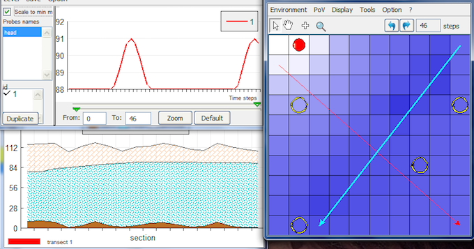
Here, the transition function of the CA is called #setAllVolumetricFluxes. Instead of having 'state' and 'bufferState', the cells use head (as 'state') and volume (as the bufferState).
So, the model calculates the diffusion of water (Q) from each cell towards its surrounded cells (or the reverse).
The latteralFlux is then multiplicated by Δt, the step duration, in order to pass from m³/s to m³/Δt as shown in the #lateralWaterDiffusion method of Plot:

lateralWaterDiffusion
"Purpose: This is the transition function of the Cellular Automata. Flux between 2 cells is calculated as:
        Fn,c = 2.T n.Tc/(Tn+Tc) . (Hn - Hc)
with T = Transmitivity = conductivity *  thickness"

This way of doing is similar for the other flows.
Then the #calculateHead method is called for each cell in order to set the new head of the cells, according to eq. 5. (#calculateHead is equivalent to the #updateState method for standard CA)

The following class diagram shows the classes of the model in its final version (Demo_Aquifer_5_rain.pcl):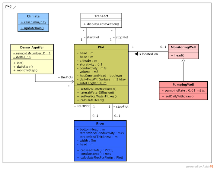

Version 1: "Demo_Aquifer.pcl"

This is the simplest version. It contains only one class: Plot. It is a 10x10 grid. A quantity of 1400 m³/day is removed from cell #2 and put to cell 99#: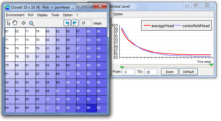
grid v1

Version 2: "Demo_Aquifer_2_transect.pcl"

In this version, 2 classes have been added to display a vertical cross-section of the grid: Transect and CrossSectionChart. From the same initialisation of version 1, a transect is added from cell #11 to cell #100 and the cross-scetion is automatically displayed. The user can also add manually as many transects as he wants.
grid V2

Version 3: "Demo_Aquifer_3_riverWells.pcl"

This version adds 3 classes: MonitoringWell (to monitor the local hydraulic head), PumpingWell (to pump water) and River. According to its head, the river may recharge or discharge the aquifers it crosses:

Gaining and losing streams. (a) Gaining stream; (b) losing stream (from Delleur 1998).

Version 4: "Demo_Aquifer_4_autoCheck.pcl"

A specific focus of the model development is the assessment of stability and convergence. A correct choice of computational time step Δt guarantees both stability and accuracy. In order to avoid chessboard effects, the Reynolds number is adjusted so as to reduce the amplitude of the oscillations of a given cell.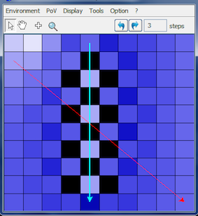

Example of auto-modification of D:

' D = 1 => deltaT = 2000  s - Daily repetition = 43 per day.'
' D = 0.9 => deltaT = 1666  s - Daily repetition = 51 per day.'
' D = 0.8 => deltaT = 1760  s - Daily repetition = 49 per day.'
' D = 0.801 => deltaT = 1790  s - Daily repetition = 48 per day.'
' D = 0.802 => deltaT = 1615  s - Daily repetition = 53 per day.'
' D = 0.803 => deltaT = 1652  s - Daily repetition = 52 per day.'
' D = 0.804 => deltaT = 1797  s - Daily repetition = 48 per day.'

Version 5: "Demo_Aquifer_5_rain.pcl"

Recharge of an aquifer usually refers to precipitation entering from the ground to the water table. The Climate is updated and each cell rechargeByRain its aquifer, only once a day.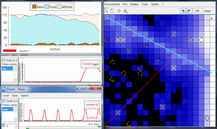

Version 6: "Demo_Aquifer_Ravazzani"

The version 6 aims at verifying the tests described in the paper by Ravazzani et al. (2011). See all the tests here.

-----------------------------------------------------------------------------------

The developed code is simple enough to facilitate its integration into other models such as land-surface models with agents.

For more information, see

Ravazzani, G., Rametta, D., & Mancini, M., 2011. Macroscopic cellular automata for groundwater modelling: A first approach. Environmental Modelling & Software, 26(5), 634-643. See paper on line

Jean Margat, Thierry Ruf, 2014. Les eaux souterraines sont-elles éternelles ? 90 clés pour comprendre les eaux souterraines. Editions Quæ,
ISSN 2261-3188 ISBN 978-2-7592-2192-9

MODFLOW 6: Harbauch A W, 2005. Modflow-2005, The U.S. Geological Survey Modular Ground-Water Model, U.S. Geological Survey Techniques and Methods 6-A16 http://water.usgs.gov/nrp/gwsoftware/modflow2005/modflow2005.html

Jacques W. Delleur, 1998. Handbook of Groundwater Engineering. Springer Science & Business Media, 1998 - 949 p, ISBN 3540647457, 9783540647454

Download the model (zipfile, 191Ko)
For more information, contact the authors.